Showing posts with label Quantitative Techniques. Show all posts

Sunday, May 29, 2022

What is the difference between "Universe" and "Population"?

Universe and Population are the two very common terms, Definitely, you know the two terms. Even though the two terms are considered as same and used interchangeably, However, both should be clearly understood in the context of statistics and research. Such as how the universe is defined? And How the population is defined in statistics and research? How do the two terms differ from each other and how do they similar to each other, that means for which case the population is said to be the universe? Here you will get the answers to all the questions. 

Universe

From the statistical point of view, the term 'universe' refers to the total of the items or units in any field of enquiry. 

For example; 

  • Total number of screws produced by a manufacturing unit in a week constitutes the universe
  • Total number of calls received by a call center in a week can be considered a universe
    Universe and Population

Population

Now turn to population. The term 'population' refers to the total of the items about which the information is desired or the set of all items or measurements in which the investigator is interested.

For example;

  • Average length of the number of screws produced in an hour
  • Average call duration of the number of calls received in an hour.

The Focus of the Population

The population focuses on a particular characteristic such as; average length of the screws or the average call duration of the calls. And the number of units possessing this characteristic constitutes the population like; a hundred thousand screws or a ten thousand calls

Now to get the average length of the number of screws produced in an hour, we take random samples of screws at different points of time in that particular hour. Same way to get the average call duration of the number of calls received in an hour, we take random samples of calls at different points of time in that hour.

When the Population and Universe are said to be the same?

But in which case, the population is considered the universe? That's the big question!  

Universe or population can refer to the same thing and can be considered synonym if the population you use while choosing your samples includes all the items of the universe.

For example: 

If you take samples from the screws produced in a week which we considered a universe, here in this case the population and universe are the same thing. Similarly, if you take samples from the calls received in a week that was also considered a universe, here again, the population and universe are the same thing.

Finite and Infinite Population

Finite Population

Now let's try to understand the finite and infinite population. 

The population or universe can be finite and infinite. The population is finite if we can enumerate or count all the items in the population.

For example:

  • The number of people living in a city
  • The number of workers in a factory
  • Number of calls received in an hour
Capital 'N' is generally used to indicate the number of items in the population.

Infinite Population
In the case of infinite population, theoretically, it is impossible to observe all the items. 

Thus in an infinite population, the number of items is infinite. We can't have any idea about the total number of items, which means we can't enumerate or count the all the items in an infinite population such as:
  • The number of stars in the sky 
  • Rivets manufactured in a company
  • Births of the insects
But the point to remember is that an infinite population of physical objects does not exist in the true sense. In spite of the fact that many such populations appear to be very very large. 

Hence for practical consideration, the infinite population is infinite because we can't count all the elements of the population in a reasonable period of time. And therefore we use the theoretical concept of infinite population as an approximation of a very large finite population.

Thursday, February 8, 2018

Video Tutorial: Process Capability | Process Improvement using Cp and Cpk Analysis

This video includes;
  1. Meaning of process capability
  2. Control limits and specification limits
  3. Relationship of limits, specifications, and distributions
  4. Process width and specification width
  5. Process capability w.r.t. specification limits (Cp)
  6. Process capability w.r.t. target (Cpk)
  7. Calculation of Cp and Cpk
  8. Analysing different cases of process for varying Cp and Cpk
  9. Process improvement
Subscribe "Shakehand with Life" YouTube Channel for more videos
Click here to download course notes

Video Tutorial: Measures of Central Tendency | Calculation of Median and Mode

This video includes;

  1. Calculation of median for individual series
  2. Calculation of median for discrete series
  3. Calculation of median for continuous series
  4. Graphical location of median
  5. Calculation of mode for individual series
  6. Calculation of mode for discrete series
  7. Calculation of mode for continuous series
  8. Graphical location of mode
  9. Empirical relation between mean, median and mode
Subscribe the "Shakehand with Life" YouTube channel for more videos
Click here to download the coursenotes


Video Tutorial: Measures of Central Tendency | Calculation of Mean

This video includes; 
  1. Meaning of individual, discrete and continuous data
  2. Calculation of mean for individual data series with help of direct and shortcut method
  3. Calculation of mean for discrete series with help of direct and shortcut method
  4. Calculation of mean for continuous series with help of direct, shortcut, and step-deviation method
Subscribe "Shakehand with Life" YouTube Channel for more video
Click here to download the coursenotes


Video Tutorial: Measures of Central Tendency | Introduction of Mean, Median and Mode

This video lecture includes;
  1. Meaning of central tendency
  2. Purpose and functions of central tendency
  3. Types of central tendency
  4. Calculation of mean median and mode
  5. Unimodal data, Bimodal data, and Multimodal data
Subscribe "Shakehand with Life" YouTube Channel to see more videos
Click here to download the coursenotes

Tuesday, September 16, 2014

Regression Analysis

Regression

Meaning 

Regression is the study of the nature of relationship between the variables so that one may be able to predict the unknown value of one variable for a known value of another variable.

Comparison between Correlation and Regression

  1. Correlation study the degree of relationship between variables while the regression study the nature of relationship between variables. 
  2. Correlation need not imply cause and effect relationship between variables whereas regression implies cause and effect relationship between variables.
  3. There may be non-sense correlation between variables whereas in case of regression there is nothing like non-sense regression.
  4. The correlation coefficient is independent of change of origin and scale but regression coefficients are independent of only change of origin but not of scale.
  5. Correlation coefficient cannot be used for prediction. But regression lines are used for prediction.

Two lines of regression

Two lines of regression
There are two lines of regression for two variables 'x' and 'y'.

Regression  equation of line Y on X

When we try to depict the change in 'y' for a given change in 'x', then the regression line of y on x is used.
The regression equation of y on x is given by
y-ybar = byx (x-xbar)
Where  byx = Cov(x,y)/Var(x)
byx is called the regression coefficient of y on x.

Regression equation of line X on Y

When we try to depict the change in 'x' for a given change in 'y'. then the regression line of x on y is used
The regression equation of x on y is given by
x-xbar = bxy(y-ybar)
Where bxy= Cov(xy)/Var(y)
bxy is called the regression coefficient of x on y

Relation between correlation and regression coefficient 

  • byx.bxy = r^2 

This implies that multiplication of both regression coefficient is equal to the square of correlation coefficient and the value of r^2 lies between 0 and 1
  • Correlation coefficient is geometric mean of both regression coefficients i.e. 

r = +/- square root( byx. bxy)


To get telephonic coaching of Correlation and Regression analysis click here

To preview of Correlation, Regression and Time series analysis e-book click here


Monday, September 15, 2014

Measures of Correlation

Measures of Correlation

Measures of Correlation
There are several method of measuring correlation between two or more variables. Some of them are mention here under.

Scatter Diagram

Scatter diagram is most popular and easy way of deciding the relation between two variables. It is a graphical method and ascertain the direction of correlation between two variables. To construct the scatter diagram take independent variable on X-Axis and dependent variable on Y Axis. Plot the graph of intersection points of two variables and decide the relation according to the scatter plot.
  1. If all the points fall on a straight line moving from left lower corner to right upper corner then it is the perfect positive correlation.
  2. If all the points fall on a straight line moving from upper left corner to right lower corner then it is a perfect negative correlation. 
  3. If all the points scattered nearby around the line then this will be high or low degree of positive and negative correlation according to the direction of line.
  4. If all the points scattered every where on the graph and no pattern will be identified then there is no correlation between the variables.

Karl Pearson's Coefficient of correlation

Scatter diagram is a graphical method of finding the correlation between two variables but it does not give the algebraic value of correlation between two variables. This become the drawback of the scatter diagram method. To overcome this Karl Pearson suggested a quantitative method of measurement of correlation which is known as the Karl Pearson coefficient of correlation denoted by (r). This gives the degree of correlation between the variables. Karl Pearson suggested the following methods to measure the coefficient of correlation. 

Deviation Method

In this method first the deviation of each variable is find out from its mean value i.e. if X and Y are two variable then the deviations are (X-Xbar) and (Y-Ybar). Now find the sum of the multiplication of the deviation. Then divide this sum by square root of sum of the square of the deviation of each variable. 

Product Moment Method

Different from deviation method the product moment method is treated the actual values of the variables multiplying the sum of the product of individual value of the variable by the number of variables and subtracting product of sum of individual values of variables. Divide this value by {square root (N. sum of square of X-square of sum of X). square root(N.sum of square of Y-square of sum of Y)}

Variance-Covariance method

In this method to find the coefficient of correlation formula of covariance and variance is used.

Spearman's Rank Correlation

Karl Pearson coefficient of correlation deal with quantitative data. But it doesn't suggest the method of treating the qualitative data. Here Spearman's Rank correlation works. This method used to find the coefficient of correlation when qualitative data is given like beauty, intelligence, sincerity, etc. There are three types of cases in Spearman's Rank Correlation method

When Ranks are given

In this case ranks have given for the qualitative data. To get the coefficient of correlation in this method we need to find the difference between the ranks then squared. Now find the sum of this squared quantities.
The formula used is
R=1-{6. Sum of D^2/(N^3-N)}
Where 'D' is difference of Ranks

When Ranks are not given 

In this case, we need to assign the ranks. Rank first is given to highest one and so on. After ranking, proceed as in the case of given ranks method.

When equal of tied ranks 

In this case calculate the average of same rank and assign this average rank to all the equal cases. Calculate a correction factor which will added in the formula as many times as the number of equal cases.

To get telephonic tutorial on Measures of correlation click here 


Thursday, September 11, 2014

Correlation Analysis

Correlation Analysis

Meaning

The correlation refers to the statistical technique used in measuring the closeness of the
Correlation Analysis
relationship between variables. e.g.
  • Price of the commodity rises as the demand for the commodity goes up.
  • Weight of a person increases with the increase in age.
  • Temperature rises with the rise in the sun light.

Definitions

  • "Correlation analysis deals with the association between two or more variables"..............Simpson and Kafka
  • "If two or more quantities vary in sympathy, so that movement in one tend to be accompanied by corresponding movements in the other, then they are said to be correlated"...................................... Conner
  • "Correlation analysis attempts to determine the degree of relationship between variables"............... Ya-Lun Chou

Uses of Correlation

  • With the help of correlation analysis, we can measure the degree of relationship in one figure between different variables like supply and price,. Income and expenditure, weight and volume manufacturing in an industry and so on..
  • We can estimate the value of one variable on the basis of the value of another,. This function is performed by regression analysis, which is based on correlation. 
  • A trader makes the estimation of costs, sales, prices etc. with the help of correlation and makes appropriate plans. 

Types of correlation

Positive Correlation

If two variables X and Y moves in same direction i.e. if one rises, other rises too and if one decline, other also decline then it is called a positive correlation e.g. money and supply

Negative Correlation

If two variables X and Y move in opposite direction i.e. if one rises, other fails, and if one fails other rises, then it is called as negative correlation e.g. demand and price.

Simple correlation 

When we try to find the relation between two variables then it is called simple correlation.

Partial correlation

Correlation among three or more variables is the study of two variables taking one variable as constant.

Multiple Correlation: 

Multiple correlation is the study of relationship among three or more variables under different conditions.

Linear Correlation 

Linear correlation is refers to the relationship between two variables such as the ratio of two variables remains constant throughout. It is best described by straight line.

Curvilinear Correlation 

It refers to the amount of change in one variable does not bear a constant ratio to the amount of change in the other variable. e.g. when every time X rises by 10%, then Y rises by 20% sometimes and sometimes by 10% and sometimes by 40% then there is no straight line relationship exist between two variable rather a curve like relation exit between the variable and it is called as curvilinear correlation. 

Degree of Correlation

The degree of correlation is expressed by the Karl Pearson's Coefficient of Correlation denoted by (r). The numerical value of (r) always between -1 and +1. On the basis of the value of (r) the Correlation has following degree of correlation.

Perfect Correlation

When the value of (r) comes -1 or +1 then it is called perfect positive or perfect negative correlation,

High Degree of Correlation

When the value of (r) comes in between either +0.75 to +1 or -0.75 to -1 then the correlation is called High degree of positive correlation or High degree of negative correlation.

Moderate Degree of Correlation 

When the value of (r) comes in between either +0.25 to +0.75 or -0.25 to -0.75 then the correlation  is called Moderate degree of positive and negative correlation.

Low degree of Correlation

When the value of (r) comes in between either 0 to +0.25 or 0 to -0.25 then the correlation is called Low degree of positive and negative correlation. 

Absence of Correlation 

When there is no correlation between the variables then the value (r) comes zero and this situation is called absence of correlation.


To get telephonic tutorial of Correlation Analysis click here


Wednesday, September 10, 2014

Standard Deviation


Standard Deviation

Calculation of Standard dispersion
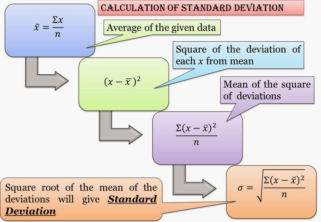
Calculation of Standard deviation
Standard deviation is defined as the square root of the arithmetic mean of the squares of the deviation of the values taken from the mean. It is denoted by small Greek letter read as ''sigma''. 

Calculation of standard deviation can understand by the fig. and mentioned below 

let 

X = X1, X2, X3, X4, ............................Xn

Xbar = (Sum of All Xn)/n
Now calculate the square of the deviation from each X from Xbar and then  calculate the mean of square of the deviations given as 
Sum(Xn-Xbar)^2/n
Now find the square root of this value and find the standard deviation of the data

Hence Standard deviation= square root(Sum(Xn-Xbar)^2)/n

Population Standard deviation

When sum of square deviation is divided by n then it is the population standard deviation

Sample Standard deviation

When sum of square deviation is divided by (n-1) then it is the sample standard deviation.

Difference between Mean deviation and standard deviation

  1. Algebraic signs of deviations (+/-) ignored while calculation mean deviation whereas in the calculation of standard deviation signs of deviations are not ignored i.e. they are taken into account .
  2. Mean deviation can be computed either from mean , median or mode. The standard deviation, on the other hand , always computed from the mean because the sum of the squares of the deviations taken from the mean is minimum.
To get Telephonic tutorials and e-book of Quantitative Techniques measure of dispersion click here


Monday, June 2, 2014

Normal curve, Area under the normal curve and control limits

Normal Curve

A very famous and common type of population distribution is known as "Normal distribution or Gaussian distribution". The data is distributed under the normal curve symmetrically. The normal curve is a symmetrical, uni modal, bell shaped with mean median and mode having the same value. Much of the variation in nature and in industry follows the frequency distribution of normal curves. The normal curve is such a good description of the variations that occur to most quality characteristics in industry that it is the basis for many quality control techniques. There is definite relationship among mean , the standard deviation and the normal curve. Normal curves with different mean but same standard deviation may cause of shift of normal curve and hence change their location as shown in fig.....
Normal curves which have same mean but different standard deviation may cause of the normal curve at the same place Normalas shown in fig.....
The fig. explained that larger the S.D. , flatter the curve (data are widely dispersed) and smaller the S.D., the more peaked the curve(data are narrowly dispersed). If the standard deviation is zero then all  values are identical to the mean and there is no curve.

The normal distribution is fully defined by the population mean and population S.D.. Also the above fig's show that these two parameters are independent. In other words a change in one parameter has no effect on the other.

Area under the normal curve

The area under the normal curve is given by the relationship of mean and standard deviation and mention below
  • 68.27%  observations are included with in the limits of "mean+/- 1Std. Dev."
  • 95.45% observations are included with in the limits of "mean+/- 2Std. Dev."
  • 99.73% observations are included with in the limits of "mean+/- 3Std. Dev."
  • 100% observations are included in between +/- infinity. this is because the normal curve never touches the X-Axis
These percentages hold true regardless of the shape of the normal curve.

The area under the normal curve is more elaborate in below fig. in which 10 over bowling spell of a bowler in one day match is shown. The Yellow balls delivered in between "mean+/- 1S.D. which is 68.27%. The Blue balls delivered between +/- 1S.D. and +/- 2 S.D. but the total of Yellow and Blue balls results 95.45% deliveries. The Red balls are delivered between +/- 2 S.D. and +/- 3 S.D. and the total delivered balls percentage will come out as 99.73%.

Normal curve and control limits of control charts

An important fact is that 99.73 %  observations fall between mean+/- 3S.D. and it becomes the base of control limits (Upper Control Limit and Lower Control Limit)  of the control charts as shown in below fig.


Monday, November 5, 2012

Introduction of Matrices

Introduction of Matrices; Quantitative Techniques; Quantitative Methods; Multiple Choice Questions (MCQ'S) based on Matrices; MBA; MDU DDE; MBA first semester;Tutorial for MBA first semester;


Friday, August 31, 2012

Previous Solved Paper, Quantitative Methods Feb. 2012. MBA Ist Sem. MDU, DDE

This paper is the collection of 70 MCQ of Quantitative Methods with free Answer Key, available on the last page of this paper. Examination Feb. 2012, MBA Ist Sem, MDU, DDE. The paper is available for free to all students of MBA, MDU, DDE,  who are going to take the  examination in Sept. 2012.

If anyone wants to solution of each question in detail then visit for the link below for Complete solution of this paper. For complete solution of  this paper  click here


Thursday, June 28, 2012

Practice Set I , 100 Multiple choice Questions of Quantitative Techniques


This paper consists of 100 multiple choice questions of different units of quantitative techniques and helpful for the students of management to score good marks in their examination of quantitative techniques. Answer key is also provided with this paper to check oneself's ability of scoring the marks in the coming examination.

To Preview and buy this practice set click here

Tuesday, June 26, 2012

Central Tendency : Mean

Mean is a very important kind of central tendency. This tutorial give you the clear idea of mean and its properties. Example illustring the problem related to the mean of discrete and continuous series.
For download this tutorial click on the top corner of this window of tutorial and press Ctrl+s and save as target. For more tutorials click here

Tuesday, October 12, 2010

Statistics of Love

Three boys saw an extremely beautiful girl . After seen the girl the boys were not able to stop themselves to propose the girl. So, the boys  approached the girl and after came to her  they  said,” Excuse us Miss, we would like to say something to  you.” 


The girl looked the boys very gently and replied, “ Please, gentlemen if you have any problem?.”

One of them said in a very soft and calm voice, “ Miss , we want to say that after having  seen you , we have some sweet –sweet feeling in our  heart for you, we think all of  us are in Love with you. Will u marry one of us?.”
Now the girl who belongs to statistical background said, “ok, gentlemen it feels very nice to heard all these, but one thing I would like to say  that can you prove it statistically? I would like to choose the best among you.”
Now the Lips of all three boys were  sealed and  they  thought that how could it be possible to prove the love statistically.
They  got back to their position and continuously thinking about this through the whole day but never forget the face of the girl.
In search of solution they went to a professor of statistics and told him about their problem.
The professor advised them, “Ask the girl to allow you to see her continuously for ten days”.
Next day on the same place , They go to the girl and asked her the same thing.
The girl replied to the boys , “she has no problem on this but they  will not try to misbehave with her at any cost”
The boys had given promise on this.
Now the boys  went to the professor and tell him that the girl allowed them  to see her for ten days .
Now professor advised them,“Note down your heart beat per minute daily for ten days while seeing the girl.”
Now the data of heart beat/min  of the boys  after ten days was like this
Day
1
2
3
4
5
6
7
8
9
10
Boy 1
98
96
92
94
95
89
79
73
92
75
Boy 2
96
88
86
82
89
90
79
75
82
78
Boy 3
78
76
74
75
77
79
76
78
79
80
After collecting the data the boys went  to the professor and show the data.
Professor calculated the averages of data of heartbeats of all three boys and find that
Average heartbeat/min
of all three boys
Boy 1
Boy 2
Boy 3
88.30
84.50
77.20
Now professor said to first boy that  show the data to the girl and tell her that your average heart beat is highest among three boys so you  are the perfect life partner for the girl as your heart is beating more than other two boys
Boys went to the girl and first boy said very confidently  by showing the data , “Miss, here is the data of our  heartbeats for ten days whenever we saw  you our  hearts were beating more than the normal and also my average heartbeat  is  more than other two boys , So I   am the best person to get marry with you.”
Girl replied in the answer of the boy, “OK, Gentleman, but I would like to analyze all the  data by my own and then I will answer you that who will be best person to get marry with me. I will answer you in next three days at  three different places individually.”
Next  three days would going to be very crucial to all three boys as they don’t know who will get the opportunity to marry with the girl.
The girl analysis the whole data by own and found the result below  
Variable
Day
Mean
Std. Dev.
Coeff. Var.
Min.
Median
Max.
Skewness
Boy1
10
88.30
9.17
10.38
73.00
92.00
98.00
-0.86
Boy2
10
84.50
6.43
7.61
75.00
84.00
96.00
 0.26
Boy3
10
77.20
1.93
2.50
74.00
77.50
80.00
-0.24

Now on next day the girl meet the first boy and said , “ No doubt that your average heart beat is more than other two boys but Std. Dev. and coff. of var.  is very high  which is 9.17, and 10.38 respectively which shows that your love to me has very high variability and very low consistency also value of skewness -0.86 shows high negative asymmetry of data and the difference between  your minimum and maximum value of  heart beat is 25 this shows that sometime you will love me with high emotions and sometime  this shows neutral behavior to me , So in all in all the data of your heartbeat is not reliable and so I cannot marry with you, I am very sorry gentleman.”  
 
Next day girl meet the  2nd boy and said, “ Your average heartbeat is also good but the Std. Dev and Coff. of Var.  are 6.43 and 7.61. No doubt both are less than in case of the first boy but still the variation of  data is quite high. It shows that your love to me also  has  high variability and low consistency. The value of skewness 0.26  shows that low  positive asymmetry of  data. The difference between your minimum and maximum value of heartbeat is 21 which means high difference of intensity of love towards me. Above all ,  your data  shows that your love is also not static to me, so gentleman I cannot go with you, Sorry.”


At last girl meet the third boy, who was looking very depressed as he had lowest average heartbeat. Girl said to the boy, “ Gentleman your heartbeat is 77.20 lowest among three but Std. Dev. and Coff. of Var. are 1.93 and 2.50 respectively which shows low variability and quite good consistency. Also the value of skewness is -0.24 is also the lowest value of asymmetry of data. The difference of  your minimum and maximum value of heartbeat is 6 which also lowest among three which means your love to me is quite static throughout the life even the intensity of love is low. Above all,  the data analysis shows you could be better life partner for me.
 
Then the Girl bent on her knees 
asked the boy.........................
To listen the answer of the girl the third boy filled with joy and  picked up the girl in his arms.
This way the girl chose the right partner for her using statistics.
From the above story we conclude that Statistics make us enough capable to take  right decisions at right time and in  right way not only in corporate life but also in our personal life.

APQP Training